


Description
This Application Note explains how to convert the raw output from an electrolytic tilt sensor into degrees.
Linear Range and Operating Range of Tilt Sensors
An electrolytic tilt sensor’s measurement range can be described in two ways: linear range and operating range. Operating range is the range over which the sensor will give a monotonic output, but otherwise has no defined characteristics (it is non-linear). Linear range is the portion of the operating range where the output is linear to within a certain percentage. Figure 1 shows the difference between the two ranges.
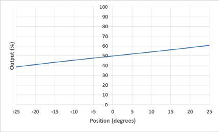
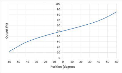
Figure 1 Linear Range (left) and Operating Range (right).
Linear Approximation
To find the tilt angle within the linear range, it is necessary to find a linear function that matches the output of the sensor. This will be the function of the line in the left graph in figure 1. This function is given below:
The raw sensor output in this formula is the sensor’s output. This is usually in counts, but other units may be used depending on how sensor output is read.
The other two values will require taking samples of the sensor at certain angles. These angles can be determined using another sensor, a digital protractor, or any other method of determining angles. The raw sensor output at 0° is just the output when the sensor is level.
The counts per degree (which is the slope of the line) is calculated using the following formula:
![]()
The linear range is obtained from the datasheet for the sensor. The raw outputs will be the sensor output at the edges of the linear range. For example, for a sensor with a linear range of ±25°, the raw outputs would be sampled at +25° and -25°. Note that these samples will only need to be taken once to create the function; converting tilt can then be done using the sampled values.
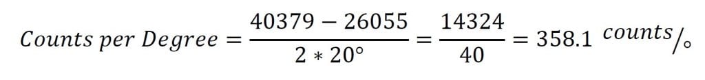
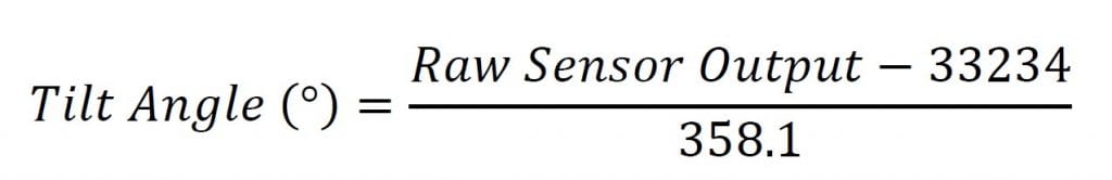
Let’s say we have an 0717-4319-99 sensor with a 16-bit (0 to 65535) output we would like to convert to degrees. This is a dual axis sensor with a linear range of ±20°. Since it is a dual axis sensor, we will need 2 formulas: one for the X axis and one for the Y axis. First, we will find the X axis formula. We start be taking samples at 0° and ±20° and find the following measurements.
X Axis Tilt at -20° = 26055
X Axis Tilt at 0° = 33234
X Axis Tilt at ±20° = 40379
Now we can use these samples to calculate the counts per degree:
The counts per degree and zero sample can then be plugged into the formula to give the conversion below:
If a Y axis measurement is necessary, follow these steps again with samples from the Y axis.
Now, whenever we have a measurement from this sensor we would like to convert to degrees, we can use this new formula. For example, if we have an X output of 29655, we can use the formula to determine the tilt angle:
![]()
Approximate Counts per Degree
Due to slight variations caused by the manufacturing process, the conversion function should be calculated for each specific sensor. However, this is not always feasible. The table below gives average counts per degree and 0° values that can be used in calculations. Note that using these values will result in less accurate measurements than creating a function for the specific sensor. All values are for a 16-bit (0-65535) output. Sensors not in the table will require the user to follow the procedure above to find a conversion.
| Sensor | Counts per Degree | Zero Degrees |
| 0703-1602-99, 0729-1765-99 | 976 | 32768 |
| 0703-0711-99 | 17582 | 32768 |
| 0717-4303-99 | 736 | 32768 |
| 0717-4304-99 | 268 | 32768 |
| 0717-4305-99 | 188 | 32768 |
| 0717-4306-99 | 188 | 32768 |
| 0717-4311-99 | 268 | 32768 |
| 0717-4313-99 | 342 | 32768 |
| 0717-4314-99 | 335 | 32768 |
| 0717-4316-99 | 756 | 32768 |
| 0717-4317-99 | 569 | 32768 |
| 0717-4318-99, 0729-1751-99, 0729-1752-99, 0729-1753-99, 0729-1754-99, 0729-1755-99, 0729-1759-99, 0729-1760-99 |
284 | 32768 |
| 0717-4319-99 | 363 | 32768 |
| 0717-4321-99 | 758 | 32768 |
| 0717-4322-99 | 594 | 32768 |
| 0737-0101-99 | 2887 | 32768 |
| 0737-1203-99 | 12765 | 32768 |
Multi-Point Interpolation
The multi-point interpolation method uses samples taken ahead of time to derive the measurement in degrees. This method’s accuracy will depend on the number and distribution of the samples; however, even taking 3 samples generally provides a better result than a linear approximation.
Sample distribution is one of the most important factors to reaching an accurate conversion. Conversions close to samples will be more accurate. Because of this, samples taken closer together will result in more accurate conversions. These samples should be taken across the entire range of the sensor. Depending on the application, they can be evenly dispersed evenly across the entire range or focused in one region where precision is necessary.
To convert a raw value to degrees, identify two reference samples. These are the two samples that are closest to the measurement in each direction. Then, find a linear approximation between the two samples and map the raw output onto this approximation. The point on this line will give the sensor’s tilt in degrees. The graph in figure 2 shows a visualization of this concept.
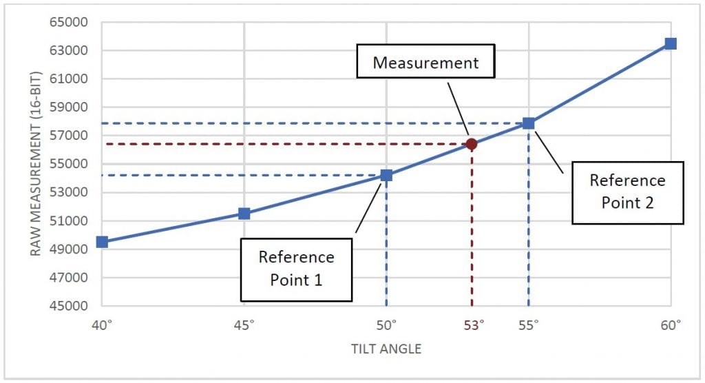
Figure 2 Graph displaying samples, reference samples, and the measurement.
The formula for this conversion is shown below.
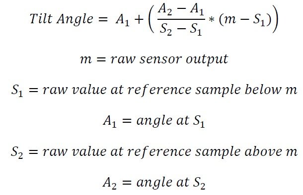
Let’s say we have a raw measurement of 56412 from a tilt sensor with a ±60° operating range. Also, suppose we already took samples at 5° intervals to use for the conversion. By comparing 56412 with the samples, we determine our two reference points will be at 50° (54213) and 55° (57878). We can then use the formula to calculate the angle:

Therefore, our final measurement is 53°.
This method can be used to convert measurements from anywhere within the sensor’s operating range to degrees. It will also achieve a better accuracy than the linear approximation. However, it requires a large number of accurate samples to achieve the best results.
Polynomial Interpolation
Polynomial interpolation can be used to achieve accurate measurements without taking many samples. This method will use samples to find a polynomial equation that will provide an accurate conversion across the operating range of the sensor.
The samples taken will be used to develop a polynomial equation that will describe the sensor output. At a minimum, you will need N-1 samples to derive a degree N polynomial. For example, 7 samples will create a degree 6 polynomial. You can also use more samples to create a lower degree polynomial, but this will generally have lower accuracy than creating a higher degree polynomial with the same points.
Any number of samples can be used, but we recommend taking at least 3 samples. Using 2 samples would work, but will result in a linear approximation. Note that there is little accuracy improvement from polynomials of degree 7 or higher.
While the polynomial can be determined manually, it is much easier to calculate it using software. One simple method is to use Microsoft Excel’s line of best fit; however, this will may not be precise enough for a usable conversion. Wolfram Alpha is a more accurate option, but the equation will still have to be solved manually. The best option is to use a programming library. For example, the Polynomial.fit() method from the NumPy Python library can be used. The code below shows how this can generate a 6th order polynomial from 7 points:
import numpy.polynomial.polynomial
coefficients = numpy.polynomial.polynomial.Polynomial.fit(
[56668, 46553, 36140, 32845, 31207, 21913, 9586], # raw values
[60, 42, 12, 0, -6, -36, -60], # corresponding angle values to the raw values
6) # order of polynomial
print(coefficients)
# Output:
# [-7.88427627e+01 2.57631617e-03 -7.71958174e-08 -1.75354175e-13
# 2.17551410e-16 -5.89635260e-21 4.45379575e-26]
Note that when using a function like this, it is important to specify the order properly. For example, 4 samples will generate a 3rd order polynomial. However, if 4 is given as the order, the library will make a random guess to create an equation. This will result in less accurate conversions.
The array returned by Polynomial.fit() are the coefficients of the polynomial. Based on the output above, the equation would be:
Angle = (4.45e-26)x6 – (5.89e-21)x5 + (2.17e-16)x4 – (1.75e-13)x3 – (7.72e-8)x2 + (2.57e-3)x1 – 78.84
This function can then be used to solve unknown angles by plugging in the raw value for x. For example, let’s say we have the function above, and have a raw measurement of 41643. We can find the angle using the following calculations:
Angle = (4.45e-26)(41643)6 – (5.89e-21)(41643)5 + (2.17e-16)(41643)4 – (1.75e-13)(41643)3 – (7.72e-8)(41643)2 + (2.57e-3)(41643)1 – 78.84
Angle = 232.264 – 738.402 + 654.227 – 12.663 – 133.868 + 107.285 – 78.842 = 30.002°
If using the NumPy library shown above, this can be done using the polyval() method.
print(numpy.polynomial.polynomial.polyval(41643, coefficients.convert(.coef))
# Output: 30.001695321007
Note that the result of this calculation is very sensitive to any change in input. For example, if the coefficients above are rounded to 3 significant digits (as written), the result of the equation is 31°. Because of this, it is important to not round any values while calculating angle with this method.