


Beschreibung
This Application Note explains how to convert the raw output from an electrolytic tilt sensor into degrees.
Linearer Bereich und Arbeitsbereich von Neigungssensoren
An electrolytic tilt sensor’s measurement range can be described in two ways: linear range and operating range. The operating range is the range over which the sensor will give a monotonic output but otherwise has no defined characteristics (it is non-linear). The linear range is the portion of the operating range where the output is linear to within a certain percentage. Figure 1 shows the difference between the two ranges.


Abbildung 1 Linearer Bereich (links) und Betriebsbereich (rechts).
Lineare Approximation
To find the tilt angle within the linear range, it is necessary to find a linear function that matches the output of the sensor. This will be the function of the line in the left graph in Figure 1. This function is given below:
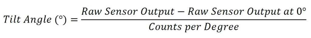
Der rohe Sensorausgang in dieser Formel ist der Ausgang des Sensors. Dies ist normalerweise in Zählungen, aber andere Einheiten können verwendet werden, je nachdem, wie die Sensorausgabe gelesen wird.
Für die beiden anderen Werte müssen Proben des Sensors in bestimmten Winkeln genommen werden. Diese Winkel können mithilfe eines anderen Sensors, eines digitalen Winkelmessers oder einer anderen Methode zur Bestimmung von Winkeln ermittelt werden. Der Rohsensorausgang bei 0° ist nur der Ausgang, wenn der Sensor waagerecht ist.
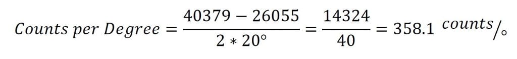
The counts per degree (which is the slope of the line) are calculated using the following formula:
![]()
The linear range is obtained from the datasheet for the sensor. The raw outputs will be the sensor output at the edges of the linear range. For example, for a sensor with a linear range of ±25°, the raw outputs would be sampled at +25° and -25°. Note that these samples will only need to be taken once to create the function; converting tilt can then be done using the sampled values.
Let’s say we have a 0717-4319-99 sensor with a 16-bit (0 to 65535) output we would like to convert to degrees. This is a dual axis sensor with a linear range of ±20°. Since it is a dual axis sensor, we will need 2 formulas: one for the X axis and one for the Y axis. First, we will find the X axis formula. We start be taking samples at 0° and ±20° and find the following measurements.
Neigung der X-Achse bei -20° = 26055
X-Achse Neigung bei 0° = 33234
X-Achse Neigung bei ±20° = 40379
Jetzt können wir diese Proben verwenden, um die Zählungen pro Grad zu berechnen:
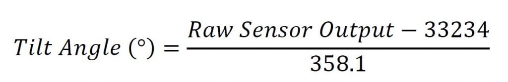
The counts per degree and zero samples can then be plugged into the formula to give the conversion below:
Wenn eine Messung der Y-Achse erforderlich ist, führen Sie diese Schritte erneut mit Proben der Y-Achse durch.
Now, whenever we have a measurement from this sensor we would like to convert to degrees, we can use this new formula.
For example, if we have an X output of 29655, we can use the formula to determine the tilt angle:
![]()
Ungefähre Zählungen pro Grad
Aufgrund von leichten Abweichungen, die durch den Herstellungsprozess verursacht werden, sollte die Umrechnungsfunktion für jeden spezifischen Sensor berechnet werden. Dies ist jedoch nicht immer machbar. Die folgende Tabelle enthält durchschnittliche Zählwerte pro Grad und 0°-Werte, die für die Berechnungen verwendet werden können. Beachten Sie, dass die Verwendung dieser Werte zu weniger genauen Messungen führt als die Erstellung einer Funktion für den spezifischen Sensor. Alle Werte beziehen sich auf einen 16-Bit-Ausgang (0-65535). Für Sensoren, die nicht in der Tabelle aufgeführt sind, muss der Benutzer das oben beschriebene Verfahren befolgen, um eine Umrechnung zu finden.
| Sensor | Zählungen pro Grad | Null-Grad |
| ApexTwo™ | 284 | 32768 |
| F203-00A-212-00 | 17582 | 32768 |
| F225-00T-003-01 | 976 | 32768 |
| 0703-0711-99 | 17582 | 32768 |
| 0703-1602-99 | 976 | 32768 |
| 0703-1603-99 | 976 | 32768 |
| 0717-4303-99 | 736 | 32768 |
| 0717-4304-99 | 268 | 32768 |
| 0717-4305-99 | 188 | 32768 |
| 0717-4306-99 | 188 | 32768 |
| 0717-4311-99 | 268 | 32768 |
| 0717-4313-99 | 342 | 32768 |
| 0717-4314-99 | 335 | 32768 |
| 0717-4316-99 | 756 | 32768 |
| 0717-4317-99 | 569 | 32768 |
| 0717-4318-99 | 284 | 32768 |
| 0717-4319-99 | 363 | 32768 |
| 0717-4321-99 | 758 | 32768 |
| 0717-4322-99 | 594 | 32768 |
| 0729-1751-99 | 284 | 32768 |
| 0729-1752-99 | 284 | 32768 |
| 0729-1753-99 | 284 | 32768 |
| 0729-1754-99 | 284 | 32768 |
| 0729-1755-99 | 284 | 32768 |
| 0729-1759-99 | 284 | 32768 |
| 0729-1760-99 | 284 | 32768 |
| 0729-1765-99 | 976 | 32768 |
| 0729-1767-99 | 284 | 32768 |
| 0729-1768-99 | 284 | 32768 |
| 0729-1769-99 | 284 | 32768 |
| 0737-0101-99 | 2887 | 32768 |
| 0737-1203-99 | 41942-57670 | 32768 |
Mehrpunkt-Interpolation
Die Mehrpunkt-Interpolationsmethode verwendet im Voraus entnommene Proben, um die Messung in Grad abzuleiten. Die Genauigkeit dieser Methode hängt von der Anzahl und der Verteilung der Stichproben ab; jedoch liefert selbst die Entnahme von 3 Stichproben im Allgemeinen ein besseres Ergebnis als eine lineare Näherung.
Sample distribution is one of the most important factors in reaching an accurate conversion. Conversions close to samples will be more accurate. Because of this, samples taken closer together will result in more accurate conversions. These samples should be taken across the entire range of the sensor. Depending on the application, they can be evenly dispersed evenly across the entire range or focused in one region where precision is necessary.
To convert a raw value to degrees, identify two reference samples. These are the two samples that are closest to the measurement in each direction. Then, find a linear approximation between the two samples and map the raw output onto this approximation. The point on this line will give the sensor’s tilt in degrees. The graph in Figure 2 shows a visualization of this concept.
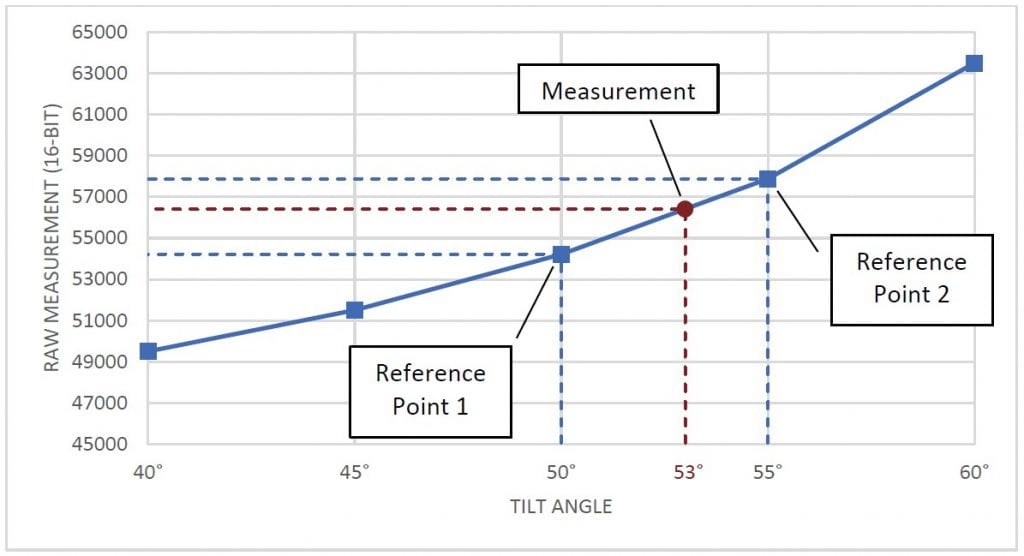
Abbildung 2 Diagramm, das Proben, Referenzproben und die Messung anzeigt.
Die Formel für diese Umrechnung ist unten dargestellt.
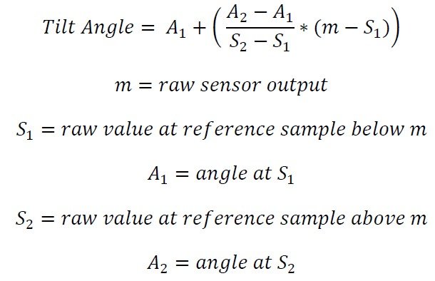
Nehmen wir an, wir haben eine Rohmessung von 56412 von einem Neigungssensor mit einem Arbeitsbereich von ±60°. Nehmen wir außerdem an, dass wir bereits Stichproben in 5°-Intervallen genommen haben, um sie für die Umrechnung zu verwenden. Durch den Vergleich von 56412 mit den Abtastwerten bestimmen wir, dass unsere beiden Referenzpunkte bei 50° (54213) und 55° (57878) liegen werden. Wir können dann die Formel verwenden, um den Winkel zu berechnen:

Daher ist unsere endgültige Messung 53°.
Diese Methode kann verwendet werden, um Messungen aus einem beliebigen Bereich innerhalb des Arbeitsbereichs des Sensors in Grad umzurechnen. Sie erreicht auch eine bessere Genauigkeit als die lineare Näherung. Sie erfordert jedoch eine große Anzahl von genauen Abtastungen, um die besten Ergebnisse zu erzielen.
Polynomiale Interpolation
Die polynomiale Interpolation kann verwendet werden, um genaue Messungen zu erzielen, ohne viele Proben zu nehmen. Diese Methode verwendet Proben, um eine Polynomgleichung zu finden, die eine genaue Umwandlung über den Betriebsbereich des Sensors liefert.
The samples taken will be used to develop a polynomial equation that will describe the sensor output. At a minimum, you will need N-1 samples to derive a degree N polynomial. For example, 7 samples will create a degree 6 polynomial. You can also use more samples to create a lower degree polynomial, but this will generally have lower accuracy than creating a
higher degree polynomial with the same points.
Es kann eine beliebige Anzahl von Stichproben verwendet werden, wir empfehlen jedoch, mindestens 3 Stichproben zu nehmen. Die Verwendung von 2 Stichproben würde funktionieren, führt aber zu einer linearen Annäherung. Beachten Sie, dass die Genauigkeit bei Polynomen vom Grad 7 oder höher kaum verbessert wird.
While the polynomial can be determined manually, it is much easier to calculate it using software. One simple method is to use Microsoft Excel’s line of best fit; however, this will may not be precise enough for a usable conversion. Wolfram Alpha is a more accurate option, but the equation will still have to be solved manually. The best option is to use a programming library. For example, the Polynomial.fit() method from the NumPy Python library can be used. The code below shows how this can generate a 6th order polynomial from 7 points:
import numpy.polynomial.polynomial
koeffizienten = numpy.polynomial.polynomial.Polynomial.fit(
[56668, 46553, 36140, 32845, 31207, 21913, 9586], # Rohwerte
[60, 42, 12, 0, -6, -36, -60], # entsprechende Winkelwerte zu den Rohwerten
6) # Ordnung des Polynoms
print(koeffizienten)
# Ausgabe:
# [-7.88427627e+01 2.57631617e-03 -7.71958174e-08 -1.75354175e-13
# 2.17551410e-16 -5.89635260e-21 4.45379575e-26]
Beachten Sie, dass es bei der Verwendung einer Funktion wie dieser wichtig ist, die Ordnung richtig anzugeben. Zum Beispiel erzeugen 4 Proben ein Polynom 3. Wenn jedoch 4 als Ordnung angegeben wird, wird die Bibliothek eine zufällige Vermutung anstellen, um eine Gleichung zu erstellen. Dies führt zu weniger genauen Umrechnungen.
The array returned by Polynomial.fit() are the coefficients of the polynomial. Based on the output above, the equation
would be:
Winkel = (4,45e-26)x6- (5,89e-21)x5+ (2,17e-16)x4- (1,75e-13)x3- (7,72e-8)x2+ (2,57e-3)x1- 78,84
Diese Funktion kann dann verwendet werden, um unbekannte Winkel zu lösen, indem der Rohwert für x eingesteckt wird. Angenommen, wir haben die obige Funktion und einen Rohwert von 41643. Wir können den Winkel mit den folgenden Berechnungen finden:
Winkel = (4,45e-26)(41643)6 - (5,89e-21)(41643)5 + (2,17e-16)(41643)4 - (1,75e-13)(41643)3 - (7,72e-8)(41643)2 + (2,57e-3)(41643)1 - 78,84
Winkel = 232,264 - 738,402 + 654,227 - 12,663 - 133,868 + 107,285 - 78,842 = 30,002°
If using the NumPy library shown above, this can be done using the polyval() method.
print(numpy.polynomial.polynomial.polyval(41643, coefficients.convert(.coef))
# Output: 30.001695321007
Note that the result of this calculation is very sensitive to any change in input. For example, if the coefficients above are rounded to 3 significant digits (as written), the result of the equation is 31°. Because of this, it is important not to round any values while calculating the angle with this method.