


설명
이 애플리케이션 노트에서는 전해 기울기 센서의 원시 출력을 각도로 변환하는 방법을 설명합니다.
선형 범위 및 틸트 센서 작동 범위
An electrolytic tilt sensor’s measurement range can be described in two ways: linear range and operating range. The operating range is the range over which the sensor will give a monotonic output but otherwise has no defined characteristics (it is non-linear). The linear range is the portion of the operating range where the output is linear to within a certain percentage. Figure 1 shows the difference between the two ranges.


그림 1 선형 범위(왼쪽) 및 작동 범위(오른쪽).
선형 근사치
To find the tilt angle within the linear range, it is necessary to find a linear function that matches the output of the sensor. This will be the function of the line in the left graph in Figure 1. This function is given below:
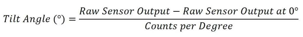
이 포뮬러의 원시 센서 출력은 센서의 출력입니다. 이는 일반적으로 계산되지만 센서 출력을 읽는 방법에 따라 다른 단위를 사용할 수 있습니다.
다른 두 값은 특정 각도에서 센서샘플을 채취해야 합니다. 이러한 각도는 다른 센서, 디지털 프로파일레이터 또는 각도를 결정하는 다른 방법을 사용하여 결정할 수 있습니다. 0°에서 원시 센서 출력은 센서가 레벨일 때 출력에 불과합니다.
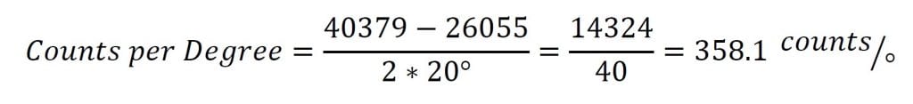
The counts per degree (which is the slope of the line) are calculated using the following formula:
![]()
The linear range is obtained from the datasheet for the sensor. The raw outputs will be the sensor output at the edges of the linear range. For example, for a sensor with a linear range of ±25°, the raw outputs would be sampled at +25° and -25°. Note that these samples will only need to be taken once to create the function; converting tilt can then be done using the sampled values.
Let’s say we have a 0717-4319-99 sensor with a 16-bit (0 to 65535) output we would like to convert to degrees. This is a dual axis sensor with a linear range of ±20°. Since it is a dual axis sensor, we will need 2 formulas: one for the X axis and one for the Y axis. First, we will find the X axis formula. We start be taking samples at 0° and ±20° and find the following measurements.
X 축 기울기 -20° = 26055
X 축 기울기 0° = 33234
x 축 틸트 ±20° = 40379
이제 이러한 샘플을 사용하여 학위당 수를 계산할 수 있습니다.
The counts per degree and zero samples can then be plugged into the formula to give the conversion below:

Y축 측정이 필요한 경우 Y 축의 샘플을 사용하여 다음 단계를 다시 따르십시오.
Now, whenever we have a measurement from this sensor we would like to convert to degrees, we can use this new formula.
For example, if we have an X output of 29655, we can use the formula to determine the tilt angle:
![]()
학위당 대략적인 개수
제조 공정으로 인한 약간의 변화로 인해 각 특정 센서에 대해 변환 기능을 계산해야 합니다. 그러나 이것이 항상 실현 가능한 것은 아닙니다. 아래 표는 계산에 사용할 수 있는 도당 평균 수와 0° 값을 제공합니다. 이러한 값을 사용하면 특정 센서에 대한 함수를 만드는 것보다 덜 정확한 측정이 발생합니다. 모든 값은 16비트(0-65535) 출력용입니다. 테이블에 없는 센서는 사용자가 위의 절차를 따라 변환을 찾아야 합니다.
| 센서 | 학위당 카운트 | 영도 |
| ApexTwo™ | 284 | 32768 |
| F203-00A-212-00 | 17582 | 32768 |
| F225-00T-003-01 | 976 | 32768 |
| 0703-0711-99 | 17582 | 32768 |
| 0703-1602-99 | 976 | 32768 |
| 0703-1603-99 | 976 | 32768 |
| 0717-4303-99 | 736 | 32768 |
| 0717-4304-99 | 268 | 32768 |
| 0717-4305-99 | 188 | 32768 |
| 0717-4306-99 | 188 | 32768 |
| 0717-4311-99 | 268 | 32768 |
| 0717-4313-99 | 342 | 32768 |
| 0717-4314-99 | 335 | 32768 |
| 0717-4316-99 | 756 | 32768 |
| 0717-4317-99 | 569 | 32768 |
| 0717-4318-99 | 284 | 32768 |
| 0717-4319-99 | 363 | 32768 |
| 0717-4321-99 | 758 | 32768 |
| 0717-4322-99 | 594 | 32768 |
| 0729-1751-99 | 284 | 32768 |
| 0729-1752-99 | 284 | 32768 |
| 0729-1753-99 | 284 | 32768 |
| 0729-1754-99 | 284 | 32768 |
| 0729-1755-99 | 284 | 32768 |
| 0729-1759-99 | 284 | 32768 |
| 0729-1760-99 | 284 | 32768 |
| 0729-1765-99 | 976 | 32768 |
| 0729-1767-99 | 284 | 32768 |
| 0729-1768-99 | 284 | 32768 |
| 0729-1769-99 | 284 | 32768 |
| 0737-0101-99 | 2887 | 32768 |
| 0737-1203-99 | 41942-57670 | 32768 |
멀티 포인트 보간
다중 점 보간 방법은 미리 취한 샘플을 사용하여 도에서 측정을 도출합니다. 이 메서드의 정확도는 샘플의 수와 분포에 따라 달라집니다. 그러나 3개의 샘플을 채취하더라도 일반적으로 선형 근사치보다 더 나은 결과를 제공합니다.
Sample distribution is one of the most important factors in reaching an accurate conversion. Conversions close to samples will be more accurate. Because of this, samples taken closer together will result in more accurate conversions. These samples should be taken across the entire range of the sensor. Depending on the application, they can be evenly dispersed evenly across the entire range or focused in one region where precision is necessary.
To convert a raw value to degrees, identify two reference samples. These are the two samples that are closest to the measurement in each direction. Then, find a linear approximation between the two samples and map the raw output onto this approximation. The point on this line will give the sensor’s tilt in degrees. The graph in Figure 2 shows a visualization of this concept.
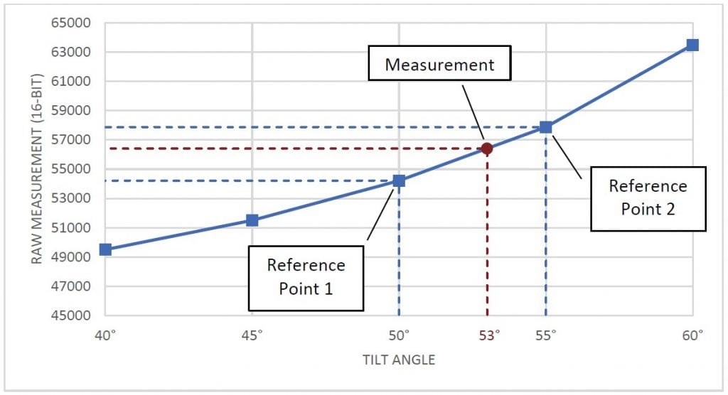
그림 2 그래프 표시 샘플, 참조 샘플 및 측정.
이 변환에 대한 공식은 다음과 같습니다.
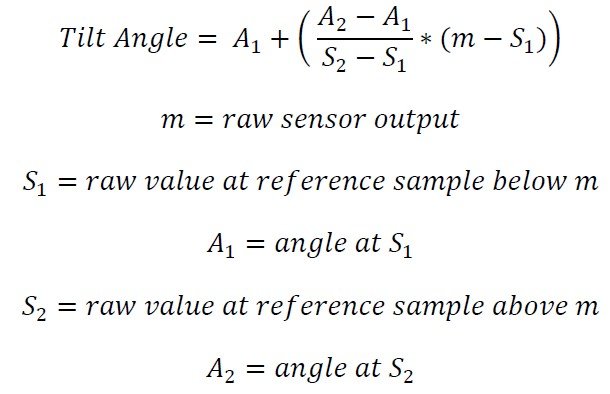
±60° 작동 범위가 있는 틸트 센서에서 56412의 원시 측정값을 가지고 있다고 가정해 봅시다. 또한 변환에 사용할 5° 간격으로 샘플을 이미 채취했다고 가정합니다. 56412와 시료를 비교하여 두 개의 기준점이 50°(54213) 및 55°(57878)에 있다고 결정합니다. 그런 다음 수식을 사용하여 각도를 계산할 수 있습니다.

따라서 최종 측정값은 53°입니다.
이 방법은 센서의 작동 범위 내의 모든 위치에서 도로 측정을 변환하는 데 사용할 수 있습니다. 또한 선형 근사치보다 더 나은 정확도를 달성할 것입니다. 그러나 최상의 결과를 얻으려면 많은 수의 정확한 샘플이 필요합니다.
다항형 보간
다항형 보간은 많은 샘플을 채취하지 않고 정확한 측정을 달성하는 데 사용될 수 있습니다. 이 메서드는 샘플을 사용하여 센서의 작동 범위에 걸쳐 정확한 변환을 제공하는 다항식 방정식을 찾습니다.
The samples taken will be used to develop a polynomial equation that will describe the sensor output. At a minimum, you will need N-1 samples to derive a degree N polynomial. For example, 7 samples will create a degree 6 polynomial. You can also use more samples to create a lower degree polynomial, but this will generally have lower accuracy than creating a
higher degree polynomial with the same points.
샘플의 수는 사용할 수 있지만, 우리는 적어도 3 샘플을 복용하는 것이 좋습니다. 2개의 샘플을 사용하면 작동하지만 선형 근사치가 발생합니다. 도 7 이상의 다항형에서 정확도가 거의 향상되지 않습니다.
While the polynomial can be determined manually, it is much easier to calculate it using software. One simple method is to use Microsoft Excel’s line of best fit; however, this will may not be precise enough for a usable conversion. Wolfram Alpha is a more accurate option, but the equation will still have to be solved manually. The best option is to use a programming library. For example, the Polynomial.fit() method from the NumPy Python library can be used. The code below shows how this can generate a 6th order polynomial from 7 points:
importnumpy.polynomial.polynomial
계수 = numpy.polynomial.polynomial.polynomial.polynomial.fit
[56668, 46553, 36140, 32845, 31207, 21913, 9586], # 원시 값
[60, 42, 12, 0, -6, -36, -60], #원시 값에 해당 각도 값
6) # 다항형 순서
인쇄(계수)
# 출력:
# #[-7.88427627e+01 2.57631617e-03 -7.71958174e-08 -1.75354175e-13
# 2.17551410e-16 -5.89635260e-21 4.45379575e-26]
이와 같은 함수를 사용할 때는 순서를 올바르게 지정하는 것이 중요합니다. 예를 들어 4개의 샘플은 3차 다항형을 생성합니다. 그러나 4가 순서로 주어지면 라이브러리는 방정식을 만들기 위해 임의의 추측을 합니다. 이렇게 하면 정확도가 떨어집니다.
The array returned by Polynomial.fit() are the coefficients of the polynomial. Based on the output above, the equation
would be:
각도 = (4.45e-26)x6 – (5.89e-21)x5 + (2.17e-16)x4 – (1.75e-13)x3 – (7.72e-8)x2 + (2.57e-3)x1 – 78.84
그런 다음 이 함수를 사용하여 x의 원시 값을 연결하여 알 수 없는 각도를 해결할 수 있습니다. 예를 들어 위의 함수를 가지고 있고 41643의 원시 측정을 한다고 가정해 보겠습니다. 다음 계산을 사용하여 각도를 찾을 수 있습니다.
각도 = (4.45e-26)(41643)6 – (5.89e-21)(41643)5 + (2.17e-16)(41643) 4 – ((41643)4 – (1.75e-13)(41643)3 – (7.72e-8)(41643)2 + (2.57e-3)(41643)1 – 78.84
각도 = 232.264 – 738.402 + 654.227 – 12.663 – 133.868 + 107.285 – 78.842 = 30.002°
If using the NumPy library shown above, this can be done using the polyval() method.
print(numpy.polynomial.polynomial.polyval(41643, coefficients.convert(.coef))
# 출력: 30.001695321007
Note that the result of this calculation is very sensitive to any change in input. For example, if the coefficients above are rounded to 3 significant digits (as written), the result of the equation is 31°. Because of this, it is important not to round any values while calculating the angle with this method.